Call:
lm(formula = wm_span ~ group, data = data_2_groups)

Residuals:
     Min       1Q   Median       3Q      Max
-3.05401 -0.61080 -0.05727  0.63912  2.96147

Coefficients:
                      Estimate Std. Error t value Pr(>|t|)
(Intercept)            3.84779    0.09567   40.22   <2e-16 ***
groupnormal attention  5.08010    0.13530   37.55   <2e-16 ***
---
Signif. codes:  0 '***' 0.001 '**' 0.01 '*' 0.05 '.' 0.1 ' ' 1

Residual standard error: 0.9567 on 198 degrees of freedom
Multiple R-squared:  0.8769,    Adjusted R-squared:  0.8762
F-statistic: 1410 on 1 and 198 DF, p-value: < 2.2e-16General Linear Model (GLM)
Form

Examples
- Attention -> WM
- Art -> Sustained attention
- ADHD -> Innatention
- Celiac disease -> Processing speed
- Intervention -> Selective attention
- Musical training -> EF
Form
𝑂𝑢𝑡𝑐𝑜𝑚𝑒 = (𝑃𝑟𝑒𝑑𝑖𝑐𝑡𝑜𝑟)
𝑂𝑢𝑡𝑐𝑜𝑚𝑒 = (𝑃𝑟𝑒𝑑𝑖𝑐𝑡𝑜𝑟) + error
Y =(𝛽) + 𝜀
Y = (𝛽0 + 𝛽1) + 𝜀
Y = (𝛽0 + 𝛽1 + 𝛽2) + 𝜀
Study effects
- Relationship
- Difference between groups
Usefulness
- Existence: statistical significance
- Size: effect size, parameter
Go

First, there were data

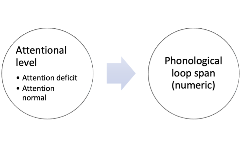
Group by attentional level

Estimate mean

Estimate relationship (difference)

GLM form
Group by attentional level

Estimate mean

Estimate relationship (difference)

GLM form

GLM form 2 vs 4 groups
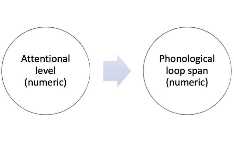
Attention and WM
Estimate relationship

Estimate relationship line

GLM form
Summary of models
Bonus
- Always GLM

GLM subtypes
